nadia-process

Overview

Perform data processing for single-cell/single-nucleus RNA-seq analysis.

nadia-process takes a matrix from nadia-quant and perform data processing steps. We use Scanpy package for most steps. They includes:

Filter cells by QC metrics
Filter genes
Doublet detection
Normalization
Feature selection (detect highly variable genes)
Dimentionality reduction (PCA)
Visualization (UMAP, T-SNE)

Users could re-run nadia-process several times to choose approriate parameters.

See: Single cell RNA-seq analysis workshop for more details.

How it works

1. Filter cells by QC metrics

There are some QC plots in the output of nadia-quant, which we can use to choose threshold to filter cells.

We should remove cells with: * high proportion of mitochondrial count * low proportion of ribosomal count * too high or too low gene count * too high or too low UMI count

See Cell filter options for more details.

2. Filter genes

There are some options to filter genes from the matrix.

We can remove genes which do not meet the minimum number of cells expressed. See –min-cell option.

We can remove mitochondrial and ribosomal genes, as their expression is mainly technical problem.

Users can provides a list of gene symbols to remove by –remove-genes option.

3. Doublet detection

Doublets detection is performed by scrublet package. It is done after filter cells and genes. Most doublet detectors simulates doublets by merging cell counts and predicts doublets as cells that have similar embeddings as the simulated doublets. It requires users to input the expected doublet rate (–expected-rate option, default 0.06).

For each barcode, scrublet will produce 2 values:

Doublet score (doublet_scores column): higher value is more likely a barcode is doublet.
Prediction (predicted_doublets column): after calculating doublet score, scrublet automatically choose a threshold to classify barcode into singlet and doublet.

If automatic threshold detection doesn’t work well, you can adjust the threshold with –min-doublet-score option.

We also create some Doublet detection plots

Finally, if –filter-doublet flag is used, then predicted doublets will be removed.

4. Dimentionality reduction

Before variable gene selection we need to normalize and logaritmize the data.

# normalize to depth 10 000
sc.pp.normalize_per_cell(adata, counts_per_cell_after=1e4)

# logaritmize
sc.pp.log1p(adata)

Next, we need to define which features/genes are important in our dataset to distinguish cell types. For this purpose, we need to find genes that are highly variable across cells, which in turn will also provide a good separation of the cell clusters.

# compute variable genes
sc.pp.highly_variable_genes(adata, min_mean=0.0125, max_mean=3, min_disp=0.5)

# subset for variable genes in the dataset
adata = adata[:, adata.var['highly_variable']]

Since each gene has a different expression level, it means that genes with higher expression values will naturally have higher variation that will be captured by PCA. This means that we need to somehow give each gene a similar weight when performing PCA (see below). The common practice is to center and scale each gene before performing PCA.

Additionally, we can use regression to remove any unwanted sources of variation from the dataset, such as n_counts’, n_genes, ‘Mito_percent’, ‘Ribo_percent’,… Users can specify the list of variables to regress by –regress option.

# regress out unwanted variables
sc.pp.regress_out(adata, regress_variables)

# scale data, clip values exceeding standard deviation 10.
sc.pp.scale(adata, max_value=10)

Finally, we perform PCA and create Dimentionality reduction plots.

# PCA
sc.tl.pca(adata, svd_solver='arpack')

5. Visualization

The UMAP implementation in SCANPY uses a neighborhood graph as the distance matrix, so we need to first calculate the graph. There are two available parameters users could specify: number of principal components to use (–n-pcs), and number of neighbors (–n-neighbors). We should choose the PCs contributing most of variance by seeing PCA variance ratio plot. To learn about --n-neighbors, click here.

sc.pp.neighbors(adata, n_pcs = n_pcs, n_neighbors = n_neighbors)
sc.tl.umap(adata)

We also run BH-tSNE.

sc.tl.tsne(adata, n_pcs = n_pcs)

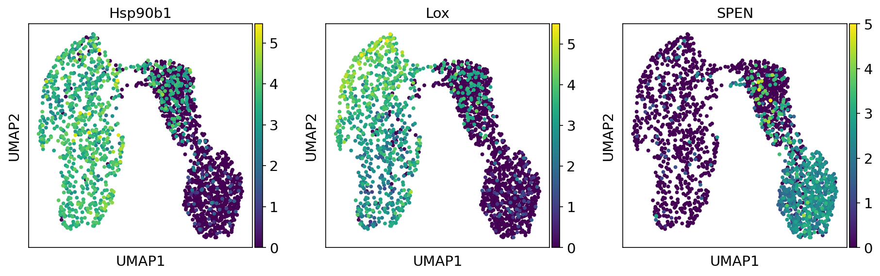
Some metadata of cells are visualized in UMAP plot, TSNE plot and Violin plot (Metadata plots). If you want to see the expression level of genes of interest in UMAP plot, you can provide the list of gene symbol in –plot-genes argument (Gene of interest plot).

Input

Gene expression matrix in either mtx format (–mtx) or h5ad format (–h5ad).

Output

Processed AnnData object

Processed AnnData object is output in h5ad format. This file could be used for further downstream analyses, such as sample integration by nadia-combine, visualization by cellxgene,…

Report

nadia-process produces a multiqc report in html format. You can download an example report

Plots

Doublet detection plots

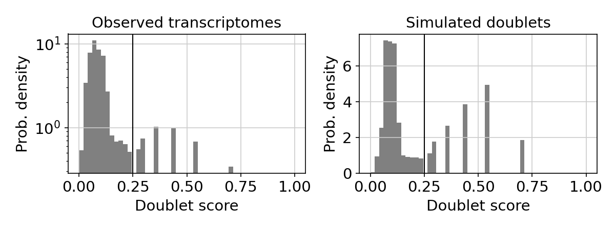
Doublet score histogram

This plot shows the doublet score histograms of observed transcriptomes and simulated doublets. The vertical line is the doublet score threshold.

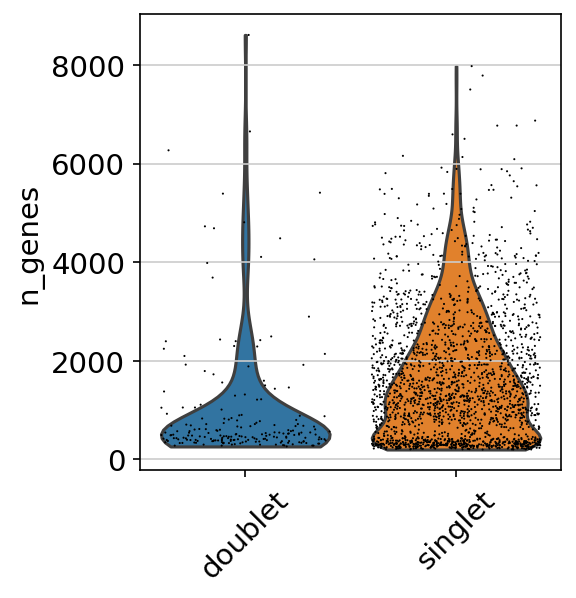
Doublet violin plot

This violin plot shows the difference in the number of genes between singlet and doublet. We can expect that doublets have more genes than singlets.

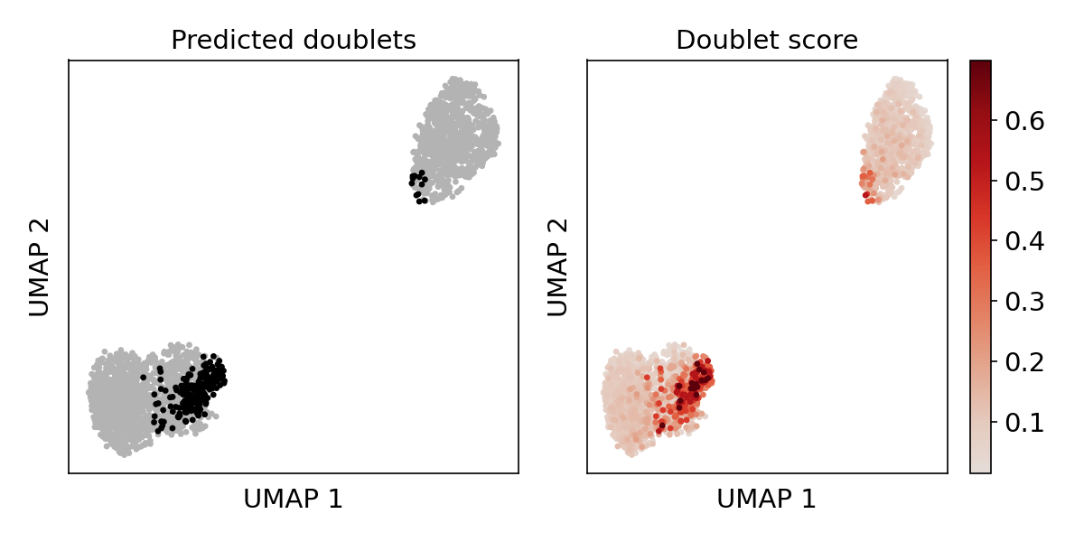
Doublet score UMAP plot

This plot shows the doublet score and the location of predicted doublet in UMAP embedding. Predicted doublets should co-localize in distinct states.

Dimentionality reduction plots

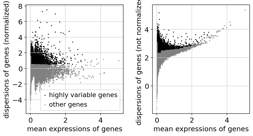
Gene dispersion plot

This plot shows the dispersion of genes by mean expression and shows genes that are filtered out.

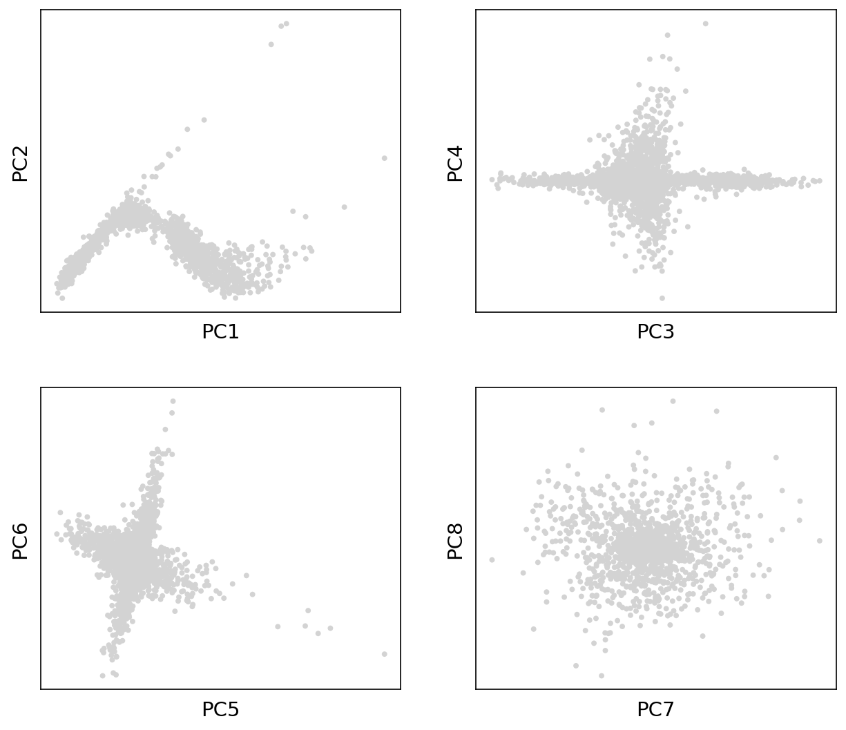
PCA plot

This plot shows the first principal components.

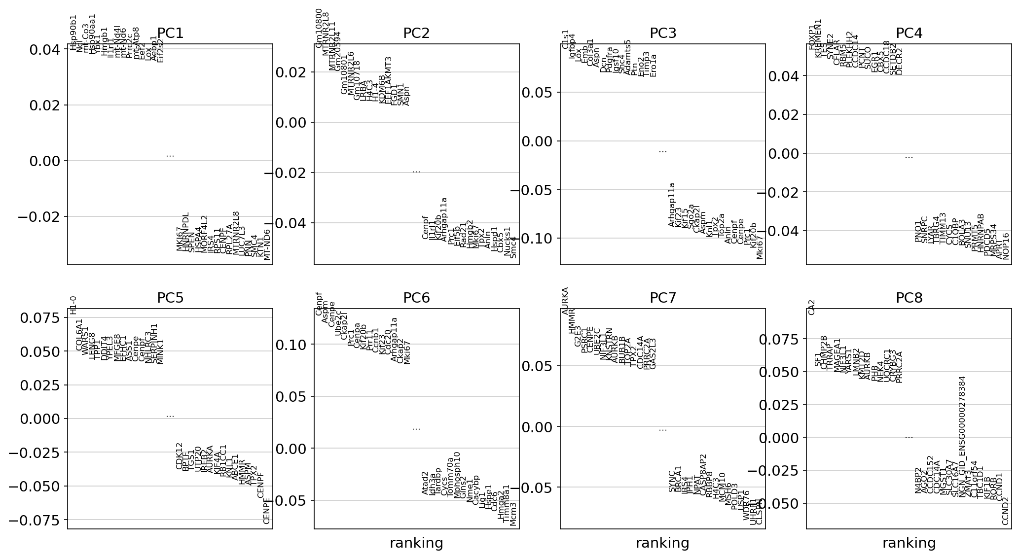
PCA loading plot

This plot identifies genes that contribute most to each PC, one can retrieve the loading matrix information.

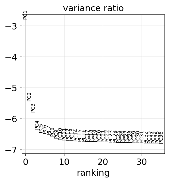
PCA variance ratio plot

This plot shows the amount of variance explained by each PC. This could be use to choose the number of PCs to use in the next steps.

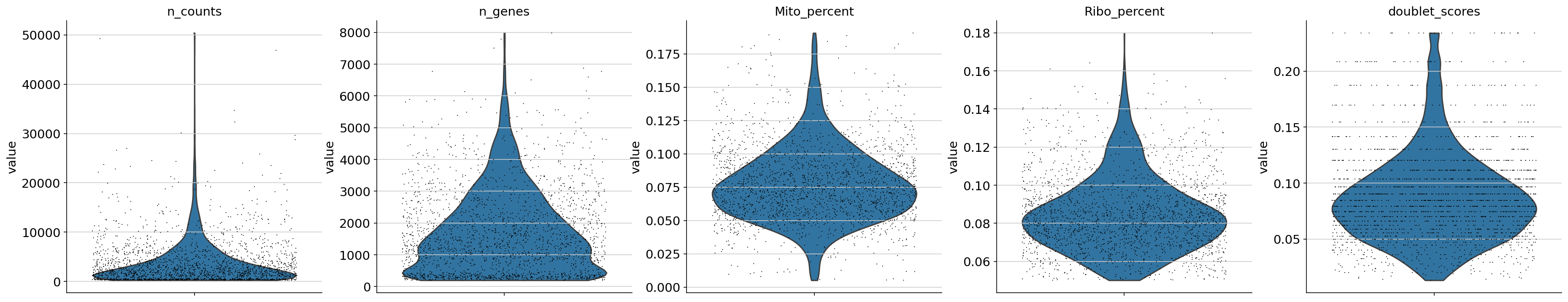
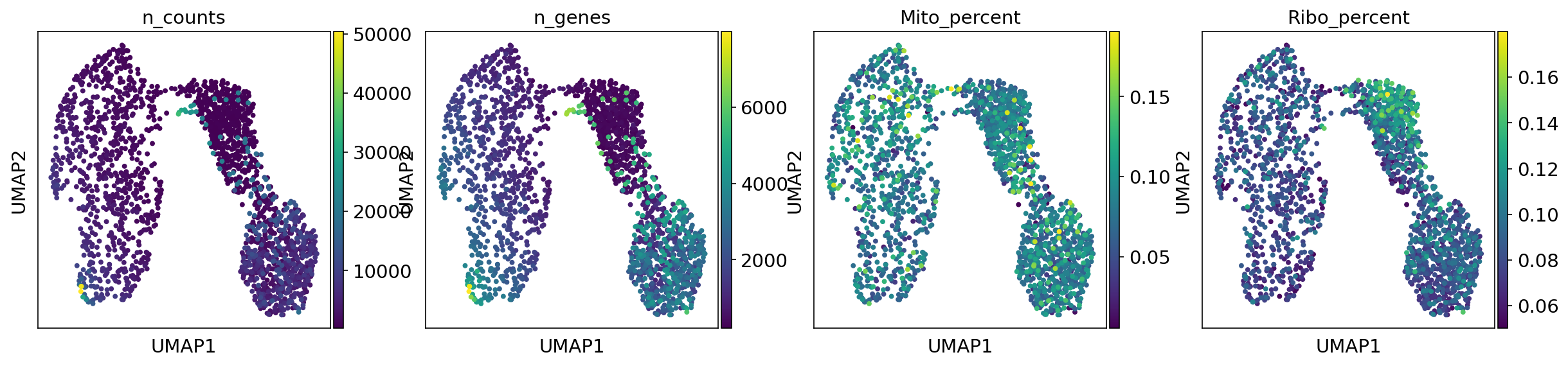
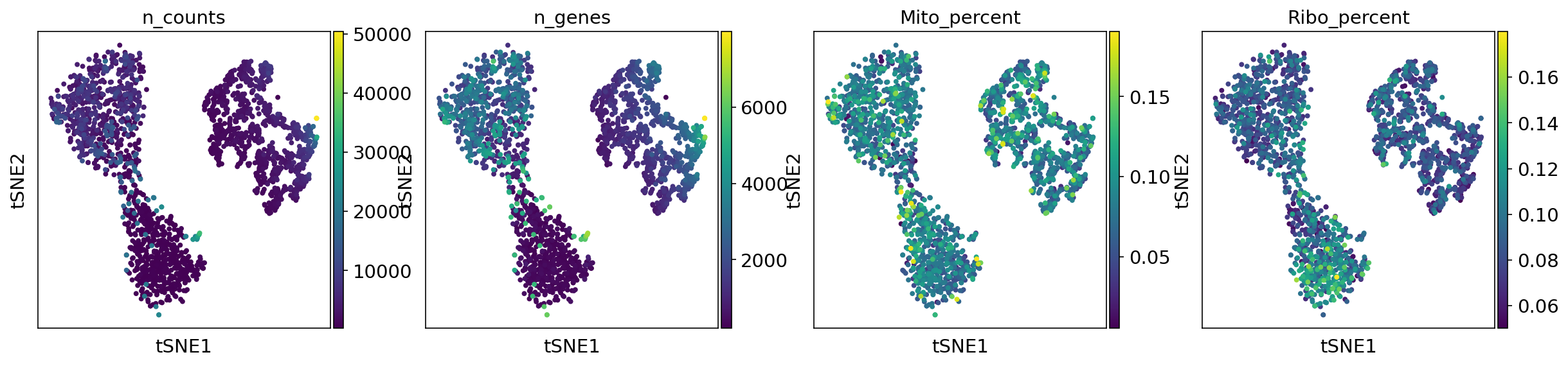
Metadata plots

Violin metadata plot

This plot shows metadata after applying all filtering.

UMAP metadata plot

T-SNE metadata plot

Gene of interest plot

Usage examples

Use h5ad file as input.

nadia-process \
    --h5ad anndata/140922_SC_4_filter.h5ad \
    -o nadiaprocess \
    --filter-doublet \
    --min-doublet-score 0.25 \
    --n-pcs 10 \
    --plot-genes Hsp90b1 Lox LOLC1 SPEN

Use mtx file as input.

nadia-process \
    --mtx MTX/140922_SC_4/filter \
    -o nadiaprocess \
    --filter-doublet \
    --n-pcs 10

Argument details

Input/Output options

`--h5ad`

Required

Path to h5ad file (AnnData object)

`--mtx`

Required

Path to matrix folder, which contains matrix.mtx, features.tsv, barcodes.tsv (gz support)

`-o`, `--outdir`

Required

Output directory

`-n`, `--name`

Sample name. It will be used for naming output files.

Required if input matrix is in mtx format. If not specified, then filename of h5ad file will be used for sample name.

Visualization options

`--regress`

Default: [‘n_counts’, ‘Mito_percent’]

List of variable to regress. Options: n_counts, n_genes, Mito_percent,…

`--n-pcs`

Default: 30

Number of Principle Components to compute UMAP and tSNE.

`--n-neighbors`

Default: 20

Number of neighbors to compute UMAP.

`--plot-genes`

List of genes of interest to plot.

nadia-process

Overview

How it works

1. Filter cells by QC metrics

2. Filter genes

3. Doublet detection

4. Dimentionality reduction

5. Visualization

Input

Output

Processed AnnData object

Report

Plots

Doublet detection plots

Doublet score histogram

Doublet violin plot

Doublet score UMAP plot

Dimentionality reduction plots

Gene dispersion plot

PCA plot

PCA loading plot

PCA variance ratio plot

Metadata plots

Violin metadata plot

UMAP metadata plot

T-SNE metadata plot

Gene of interest plot

Usage examples

Argument details

Input/Output options

--h5ad

--mtx

-o, --outdir

-n, --name

Cell filter options

--mito

--max-mito

--ribo

--min-ribo

--min-gene

--max-gene

--min-umi

--max-gene

Doublet filter options

--filter-doublet

--expected-rate

--min-doublet-score

Gene filter options

--min-cell

--remove-mito

--remove-ribo

--remove-genes

Visualization options

--regress

--n-pcs

--n-neighbors

--plot-genes

`--h5ad`

`--mtx`

`-o`, `--outdir`

`-n`, `--name`

`--mito`

`--max-mito`

`--ribo`

`--min-ribo`

`--min-gene`

`--max-gene`

`--min-umi`

`--max-gene`

`--filter-doublet`

`--expected-rate`

`--min-doublet-score`

`--min-cell`

`--remove-mito`

`--remove-ribo`

`--remove-genes`

`--regress`

`--n-pcs`

`--n-neighbors`

`--plot-genes`